
How to Build a Machine Learning Model to Identify Credit Card Fraud in 5 Steps
I will walk through the 5 steps to building a supervised machine learning model. Below is a an outline of the five steps.


Claudia
A Hands-on Modeling Guide using a Kaggle Dataset
With the surge in e-commerce and digital transactions, identity fraud is has also risen to affect millions of people every year.
In 2019, fraud losses in the US alone were estimated to be at around US$16.9 billion, a substantial portion of which includes losses from credit card fraud¹.
In addition to strengthening cybersecurity measures, financial institutions are increasingly turning to machine learning to identify and reject fraudulent transactions when they happen, so as to limit losses.
I came across a credit card fraud dataset on Kaggle and built a classification model to predict fraudulent transactions. In this article, I will walk through the 5 steps to building a supervised machine learning model. Below is a an outline of the five steps:
- Exploratory Data Analysis
- Train-test split
- Modeling
- Hyperparameter Tuning
- Evaluating Final Model Performance
I. Exploratory Data Analysis (EDA)
When starting a new modeling project, it is important to start with EDA in order to understand the dataset.
In this case, the credit card fraud dataset from Kaggle contains 284,807 rows with 31 columns. This particular dataset contains no nulls, but note that this may not be the case when dealing with datasets in reality.
Our target variable is named class, and it is a binary output of 0’s and 1’s, with 1’s representing fraudulent transactions and 0’s as non-fraudulent ones.
The remaining 30 columns are features that we will use to train our model, the vast majority of which have been transformed using PCA and thus anonymized, while only two (time and amount) are labeled.
I.a. Target Variable
Our dataset is highly imbalanced, as the majority of rows (99.8%) in the dataset are non-fraudulent transactions and have a class = 0. Fraudulent transactions only represent ~0.2% of the dataset.
This class imbalance problem is common with fraud detection, as fraud (hopefully) is a rare event.
Because of this class imbalance issue, our model may not have enough fraudulent examples to learn from and we will mitigate this by experimenting with sampling methods in the modeling stage.
I.b. Features
To get a preliminary look at our features, I find seaborn’s pairplot function to be very useful, especially because we can plot out the distributions by the target variable if we introduce thehue='class' argument.
Below is a plot showing the first 10 features in our dataset by label, with orange representing 0 or non-fraudulent transactions and blue representing 1 or fraudulent transactions.

Pairplots of first ten features in dataset by target variable value.
As you can see from the pairplot, the distributions of some features differ by label, giving an indication that these features may be useful for the model.
II. Train-Test Split
Since the dataset has already been cleaned, we can move on to split our dataset into the train and test sets. This is an important step as you cannot effectively evaluate the performance of your model on data that it has trained on!
I used scikit-learn’s train_test_split function to split 75% of our dataset as the train set and the remaining 25% as the test set.
It is important to note that I set the stratify argument to be equal to the label or y in the train_test_split function to make sure there are proportional examples of our label in both the train and test sets.
Otherwise, if there were no examples where the label is 1 in our train set, the model would not learn what fraudulent transactions are like.
Likewise, if there were no examples where the label is 1 in our test set, we would not know how well the model would perform when it encounters fraud.
X_train, X_test, y_train, y_test = train_test_split(X, y, shuffle=True, stratify=y)
III. Modeling
Since our dataset is anonymized, there is no feature engineering to be done, so the next step is modeling.
III.a. Choosing an ML Model
There are different classification models to choose from, and I experimented with building simple models to pick the best one that we will later tune the hyperparameters of to optimize.
In this case, I trained a logistic regression model, random forest model and XGBoost model to compare their performances.
Due to class imbalance, accuracy is not a meaningful metric in this case. Instead I used AUC as the evaluation metric, which takes on values between 0 and 1.
The AUC measures the probability that the model will rank a random positive example (class = 1) higher than a random negative example.
To evaluate model performances, I used stratified K-Fold Cross Validation to stratify sampling by class label, since our dataset is highly imbalanced. Using the model AUC scores, I made a boxplot to compare the ranges of AUC scores by model.
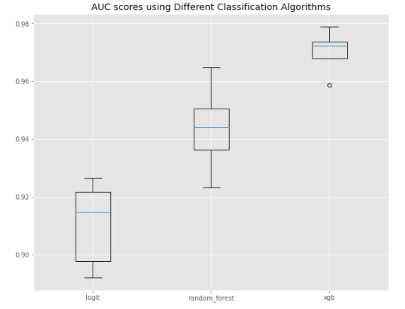
Boxplots of AUC scores of different Classification Models
Not surprisingly, XGBoost appears to be the best model of our three choices.
The median AUC score of the XGBoost model is 0.970, compared to 0.944 for that of the random forest model and 0.911 for that of the logistic regression model. So, I selected XGboost as my model of choice going forward.
III.b. Compare Sampling Methods
As mentioned previously, I also experimented with different sampling techniques to deal with the class imbalance issue. I tried outimblearn's random oversampling, random undersampling and SMOTE functions:
- Random oversampling samples the minority class with replacement until a defined threshold, which I left at the default of 0.5, so our new dataset has a 50/50 split between labels of 0’s and 1’s.
- Random undersampling samples the majority class, without replacement by default but you can set it to sample with replacement, until our dataset has a 50/50 split between labels of 0’s and 1’s.
- SMOTE (Synthetic Minority Oversampling Technique) is a data augmentation method that randomly selects an example from the minority class, finds k of its nearest neighbours (usually k=5), chooses a random neighbour and creates a synthetic new example in the feature space between this random neighbour and the original example.
I used the Pipeline function fromimblearn.pipeline to avoid leakage, then used stratified K-Fold Cross Validation to compare performances of XGBoost models with the three different sampling techniques listed above.
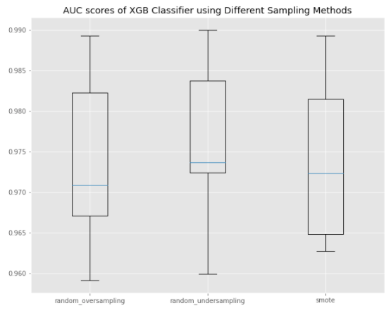
Comparing AUC scores of XGBoost Models using Different Sampling Methods
The median AUC scores of the three sampling methods are quite close at between 0.974 to 0.976. In the end, I chose SMOTE because of the smaller range in AUC scores.
IV. Hyperparameter Tuning
I chose to use Bayesian hyperparameter tuning with a package called hyperopt, because it is faster and more informed than other methods such as grid search or randomized search. The hyperparameters that I wanted to tune for my XGBoost model were:
- max_depth: maximum depth of a tree; values between 4 to 10.
- min_child_weight: minimum sum of weights of samples to form a leaf node or the end of a branch; values between 1 to 20.
- subsample: random sample of observations for each tree; values between 0.5 to 0.9.
- colsample_bytree: random sample of columns or features for each tree; values between 0.5 to 0.9.
- gamma: minimum loss reduction needed to split a node and used to prevent overfitting; values between 0 and 5.
- eta: learning_rate; values between 0.01 and 0.3.
To use hyperopt, I first set up my search space with hyperparameters and their respective bounds to search through:
space = {
'max_depth': hp.quniform('max_depth', 4, 10, 2),
'min_child_weight': hp.quniform('min_child_weight', 5, 30, 2),
'gamma': hp.quniform('gamma', 0, 10, 2),
'subsample': hp.uniform('subsample', 0.5, 0.9),
'colsample_bytree': hp.uniform('colsample_bytree', 0.5, 0.9),
'eta': hp.uniform('eta', 0.01, 0.3),
'objective': 'binary:logistic',
'eval_metric': 'auc'
}
Next, I defined an objective function to minimize that will receive values from the previously defined search space:
def objective(params):
params = {'max_depth': int(params['max_depth']),
'min_child_weight': int(params['min_child_weight']),
'gamma': params['gamma'],
'subsample': params['subsample'],
'colsample_bytree': params['colsample_bytree'],
'eta': params['eta'],
'objective': params['objective'],
'eval_metric': params['eval_metric']}
xgb_clf = XGBClassifier(num_boost_rounds=num_boost_rounds, early_stopping_rounds=early_stopping_rounds, **params)
best_score = cross_val_score(xgb_clf, X_train, y_train, scoring='roc_auc', cv=5, n_jobs=3).mean()
loss = 1 - best_score
return loss
The best hyperparameters returned are listed below and we will use this to train our final model!
best_params = {'colsample_bytree': 0.7,
'eta': 0.2,
'gamma': 1.5,
'max_depth': 10,
'min_child_weight': 6,
'subsample': 0.9}
V. Evaluation of Final Model Performance
To train the final model, I used imblearn's pipeline to avoid leakage. In the pipeline, I first used SMOTE to augment the dataset and include more positive classes for the model to learn from, then trained a XGBoost model with the best hyperparameters found in step IV.
final_model = imblearn.pipeline.Pipeline([
('smote',SMOTE(random_state=1)),
('xgb', XGBClassifier(num_boost_rounds=1000,
early_stopping_rounds=10,
**best_params))])
V.a. Metrics
Below are some metrics to evaluate the performance of the final model:
AUC
The AUC score of the final model is 0.991! This indicates that our final model is able to rank order fraud risk quite well.
Classification Report

Classification Report of Test Set
Precision
True Positives/(True Positives + False Positives)
Precision for class 0 is 1, indicating that all items labeled as belonging to class 0 are indeed non-fraudulent transactions.
Precision for class 1 is 0.86, meaning that 86% of items labeled as class 1 are indeed fraudulent transactions. In other words, the final model correctly predicted 100% of non-fraudulent transactions and 86% of fraudulent transactions.
Recall
True Positives/(True Positives + False Negatives)
Recall for class 0 is 1, meaning that all non-fraudulent transactions were labeled as such, i.e. belonging to class 0.
Recall for class 1 is 0.9, so 90% of fraudulent transactions were labeled as belonging to class 1 by our final model. This means that the final model is able to catch 90% of all fraudulent transactions.
F1 score
2 * (Recall * Precision)/(Recall + Precision)
The F1 score is a weighted harmonic mean of precision and recall. The F1 score of the final model predictions on the test set for class 0 is 1, while that for class 1 is 0.88.
V.b. Feature Importances
To understand the model, it is useful to look at the Shap summary and feature importances plots.
Unfortunately, most features have been anonymized in this dataset, but the plots show that v14, v4 and v12 are the top 3 most important features in the final model.
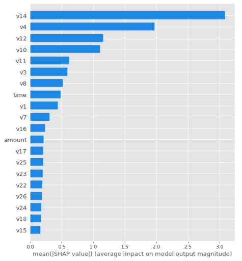
Feature Importances Plot for Final XGBoost Model
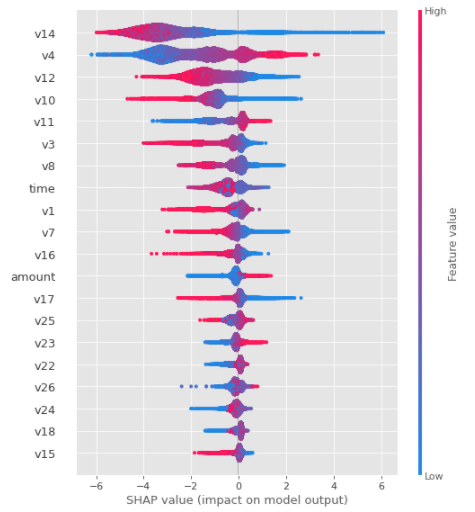
Shap Summary Plot of Test Set for Final XGBoost Model
Final Thoughts
In merely five steps, we built an XGBoost model capable of predicting whether a transaction is fraudulent or not based on the 30 features provided in this dataset.
Our final model has an AUC score of 0.991, which is incredibly high! However, it is worth noting that this was done with a pre-cleaned (and manipulated) dataset.
In reality, feature engineering is a vital step in modeling but we did not have the chance to do so here due to limits of working with an anonymized dataset.
I hope that this hands-on modeling exercise using a real dataset helped you better understand the mechanics behind creating a machine learning model to predict fraud.
I am very curious to know what the anonymized features were, especially the most predictive ones. If you have any ideas on what they could be, please comment below!
To see the code, please check out my jupyter notebook file on Github. Thank you!
References
Originally published here!
Upvote
Claudia

Related Articles