In this article, we will have a code walkthrough of an end-to-end data science project to develop, build and deploy ML powered solution

Introduction

This is a multiclass classification project to classify the severity of road accidents into three categories. This project is based on real-world data, and the dataset is also highly imbalanced. There are three types of injuries: minor, severe, and fatal.

Road accidents are the major cause of unnatural deaths around the world. To reduce accidents and fatalities, all governments work hard to raise awareness about the rules and regulations that must be followed when driving a vehicle on the road.

In this article, we will look at the end-to-end project with source code to develop a machine-learning solution to predict the severity of road accidents to take necessary precautions by the investigation agency. So let’s start with the project description and problem statement.

Note: This article was published on Analytics Vidhya’s Blogs on 14th January. link to the original published article can be found here

Project description

This data set was collected from Addis Ababa Sub-city, Ethiopia, police departments for students’ master’s research work. The data set has been prepared from manual records of road traffic accidents for the years 2017–20. All the sensitive information has been excluded during data encoding, and finally, it has 32 features and 12316 instances of an accident. Then it is preprocessed for the identification of major causes of the accident by analyzing it using different classification algorithms. Machine learning models are evaluated and thereafter deployed on a cloud-based platform in order to make them usable for end users.

Problem statement

The target feature is “Accident_severity,” which is a multi-class variable. The task is to classify this variable based on the other 31 features step-by-step by going through each data science process and task. Your metric for evaluation will be your “F1 score.”

Prerequisites

This is an intermediate-level project with an imbalanced multiclass classification problem. some of the prerequisites for this project.

• Understanding of classification machine learning algorithms is required.
• Knowledge of the Python programming language and python frameworks like Pandas, NumPy, Matplotlib, and Scikit-Learn, as well as the basics of streamlit library, is required.

Dataset description

1. Time — time of the accident (in 24 hours format)
2. Day_of_week — A day when an accident occurred
3. Age_band_of_driver —The age group of the driver
4. Sex_of_driver — Gender of driver
5. Educational_level — Driver’s highest education level
6. Vehical_driver_relation — What’s the relation of a driver with the vehicle
7. Driving_experience — How many years of driving experience the driver has
8. Type_of_vehicle — What’s the type of vehicle
9. Owner_of_vehicle — Who’s the owner of the vehicle
10. Service_year_of_vehicle — The last service year of the vehicle
11. Defect_of_vehicle — Is there any defect on the vehicle or not?
12. Area_accident_occured — Locality of an accident site
13. Lanes_or_Medians — Are there any lanes or medians at the accident site?
14. Road_allignment — Road alignment with the terrain of the land
15. Types_of_junction — Type of junction at the accident site
16. Road_surface_type — A surface type of road
17. Road_surface_conditions — What was the condition of the road surface?
18. Light_conditions — Lighting conditions at the site
19. Weather_conditions — Weather conditions
20. Type_of_collision — What is the type of collision
21. Number_of_vehicles_involved — Total number of vehicles involved in an accident
22. Number_of_casualties — Total number of casualties
23. Vehicle_movement — How the vehicle was moving before the accident occurred
24. Casualty_class — A person who got killed during an accident
25. Sex_of_casualty — What the gender of a person who got killed
26. Age_band_of_casualty — Age group of casualty
27. Casualty_severtiy — How severely the casualty was injured
28. Work_of_casualty — What was the work of the casualty
29. Fitness_of_casualty — Fitness level of casualty
30. Pedestrain_movement — Was there any pedestrian movement on the road?
31. Cause_of-accident — What was the cause of an accident?
32. Accident_severity — How severe an accident was? (Target variable)

So far, we have understood the problem statement and data descriptions. Now we will look at the end-to-end code implementations to solve predictive analytics problems and deploy machine learning solutions on the streamlit cloud.

Data understanding

Now that we have looked at the problem statement and data description, we will start loading the dataset into our development environment and start analyzing the data to find critical insights for the data preparation and modeling stages.

Source of the dataset — Click Here

Kaggle dataset link — Click Here

1. Import the dataset

I have used a Kaggle environment to work on this project. You can use this dataset in your local environment or any preferred cloud-based IDE to complete work on this project by following the step-by-step code.

# importing pandas
import pandas as pd
# using pandas read_csv function to load the dataset
df = pd.read_csv("/kaggle/input/road-traffic-severity-classification/RTA Dataset.csv")
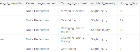
df.head()

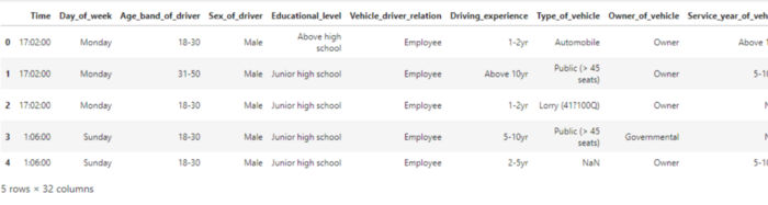
the output of the code

Note: Due to the large dataset, the output of the above code is not fully visible in a screenshot.

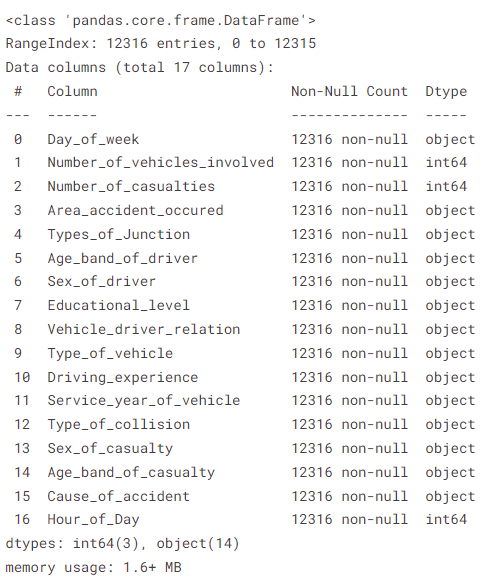
2. Metadata of the dataset

# print the dataset information
df.info()

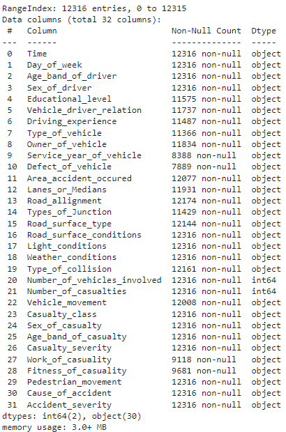
the output of the code

The above method shows metadata information such as non-null values, datatypes of each column, the number of rows and columns present in the dataset, and the memory usage of the dataset.

3. Find the number of missing values present in each column

# Find the number of missing values present in each column
df.isnull().sum()

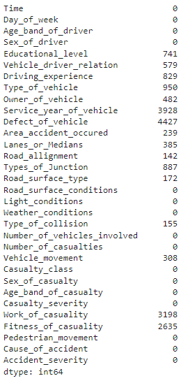
the output of the above code

The method shows us how many missing values there are in each column. “Defect_of_Vehicle” shows the highest number of missing values, which is 4427 out of 12316 instances.

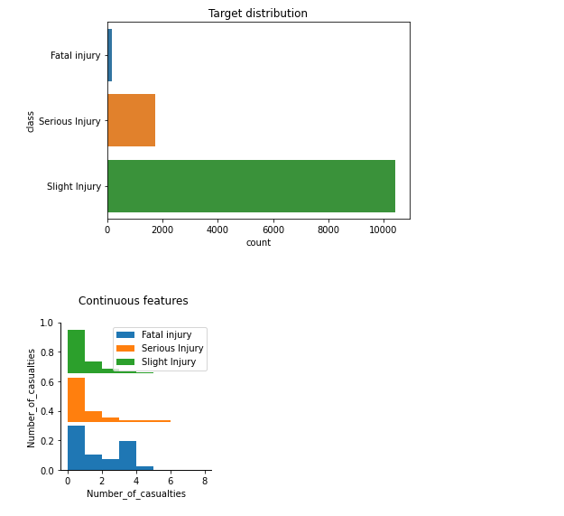
4. Target variable classes distribution and visualization

# target variable classes counts and bar plot
print(df['Accident_severity'].value_counts())
df['Accident_severity'].value_counts().plot(kind='bar')

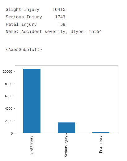
the output of the above code

As we saw earlier in the problem statement, target variable classes are highly imbalanced, and we will solve this problem during the data preparation stage to develop accurate and generalized machine learning models.

5. Exploratory data analysis of the dataset

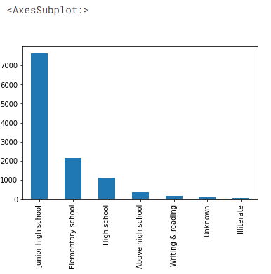
Let’s find out the education levels of drivers

# Education levels of car drivers
df['Educational_level'].value_counts().plot(kind='bar')

the output of the dataset

We can see more than 7000 drivers are having education up to junior high school and only a fraction of drivers are having education above high school.

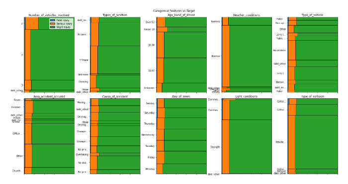
• Auto data visualization using the ‘dabl’ library

# Visualizing dataset using dabl library
dabl.plot(df, target_col='Accident_severity')

the output of the above code

the output of the above code

Using just one line of code, we can visualize the relationships between input features and a target variable. From our analysis so far, we can derive the following insights:

• More the Number of casualties, the higher the chances of fatal injuries at the accident site
• More the vehicles involved higher the chances of Serious injury
• Light_conditions being darkness can cause higher serious injury
• Data is highly imbalanced
• Features like area_accident_occured, Cause_of_accident, Day_of_week, type_of_junction seem to be essential features causing fatal injuries
• Road_surface and road conditions do not affect fatal or serious accidents apparently

(Note: I will attach a github repository link of this project at the end of this article, so you can find detailed information about the code)

• Association between the ‘road surface type’ column and target ‘accident severity’

# plot the bar plot of road_surface_type and accident severity feature
plt.figure(figsize=(6,5))
sns.countplot(x='Road_surface_type', hue='Accident_severity', data=df)
plt.xlabel('Rode surafce type')
plt.xticks(rotation=60)
plt.show

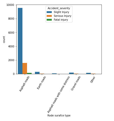
the output of the above code

We can learn that most accidents happened on “asphalt roads” in our dataset, followed by “earth roads.” Here we can say that most fatal injuries happen on asphalt roads, so they might not be a significant variable to predict the target class.

Now, based on the above findings, we will preprocess the raw data for modeling and evaluation purposes.

Data preparation

We will start pre-processing the dataset by changing the “Time” column datatype to the “datetime” datatype. We will then extract the hour of the day feature to prepare the data for modeling.

# convert object type column into datetime datatype column
df['Time'] = pd.to_datetime(df['Time'])
# Extrating 'Hour_of_Day' feature from the Time column
new_df = df.copy()
new_df['Hour_of_Day'] = new_df['Time'].dt.hour
n_df = new_df.drop('Time', axis=1)
n_df.head()

the output of the above code

Missing value treatment

By this time, we would have a subset of features to be selected for further processing based on the insights gained from the previous stage. We will select a subset of features and then treat the missing values using the “fillna()” method of the Pandas library.

In our context, we will handle missing values by filling in “unknown” as a value, assuming missing values might not have been found during the investigation.

# NaN are missing because service info might not be available, we will fill as 'Unknowns'
feature_df['Service_year_of_vehicle'] = feature_df['Service_year_of_vehicle'].fillna('Unknown')
feature_df['Types_of_Junction'] = feature_df['Types_of_Junction'].fillna('Unknown')
feature_df['Area_accident_occured'] = feature_df['Area_accident_occured'].fillna('Unknown')
feature_df['Driving_experience'] = feature_df['Driving_experience'].fillna('unknown')
feature_df['Type_of_vehicle'] = feature_df['Type_of_vehicle'].fillna('Other')
feature_df['Vehicle_driver_relation'] = feature_df['Vehicle_driver_relation'].fillna('Unknown')
feature_df['Educational_level'] = feature_df['Educational_level'].fillna('Unknown')
feature_df['Type_of_collision'] = feature_df['Type_of_collision'].fillna('Unknown')
# features information
feature_df.info()

the output of the dataframe

As we can see, our feature set now has zero null values compared to the previous raw dataset. Let’s move on to the other data pre-processing steps now.

One-Hot encoding using ‘get_dummies()’ method

Pandas’ ‘get_dummies()’ can be used to convert categorical columns into numerical features. let’s see the code snippet below:

# Categorical features to encode using one hot encoding 
features = ['Day_of_week','Number_of_vehicles_involved','Number_of_casualties','Area_accident_occured',
           'Types_of_Junction','Age_band_of_driver','Sex_of_driver','Educational_level',
           'Vehicle_driver_relation','Type_of_vehicle','Driving_experience','Service_year_of_vehicle','Type_of_collision',
           'Sex_of_casualty','Age_band_of_casualty','Cause_of_accident','Hour_of_Day']
# setting input features X and target y 
X = feature_df[features]  # here features are selected from 'object' datatype
y = n_df['Accident_severity']
# we will use pandas get_dummies method for on-hot encoding
encoded_df = pd.get_dummies(X, drop_first=True)
encoded_df.shape
-----------------------------------[Output]-----------------------------------
(12316, 106)

As a result of the encoding, we now have 106 columns in the encoded dataframe, which we will further preprocess to keep only significant features for modeling purposes.

Target encoding using ‘LabelEncoder()’ method

# import labelencoder from sklearn.preprocessing
from sklearn.preprocessing import LabelEncoder
# create labelencoder object
lb = LabelEncoder()
lb.fit(y)
y_encoded = lb.transform(y)
print("Encoded labels:",lb.classes_)
y_en = pd.Series(y_encoded)
-----------------------------------[Output]----------------------------------
Encoded labels: ['Fatal injury' 'Serious Injury' 'Slight Injury']

Now, we have “encoded_df” as an encoded dataframe object and “y_en” as an encoded target column to further select “Kbest” features and handle an imbalanced dataset.

Feature selection using the ‘Chi2’ Statistic

# feature seleciton method using chi2 for categorical output, categorical input
from sklearn.feature_selection import SelectKBest, chi2
fs = SelectKBest(chi2, k=50)
X_new = fs.fit_transform(encoded_df, y_en)
# Take the selected features
cols = fs.get_feature_names_out()
# convert selected features into dataframe
fs_df = pd.DataFrame(X_new, columns=cols)

We are selecting the top 50 features out of 106 features from the encoded dataframe and storing them in a new dataframe object called “fs_df.” The “Chi2” statistic is used when the target feature is a categorical variable, and the “Pearson’s coefficient” is used when the target feature is a continuous variable. Now let’s upsample the dataset to balance categorical features.

Imbalance data treatment using the ‘SMOTENC’ technique

The scikit-learn library has an extension library called “Imbalanced-learn,” which has various methods to handle imbalanced data. (Official documentation — Click Here).

To upsample and minority class samples, we will use the “Synthetic Minority Over-sampling Technique for Nominal and Continuous” (SMOTENC) techniques in our project. This method is designed for categorical and continuous features to accurately upsample the dataset.

# importing the SMOTENC object from imblearn library 
from imblearn.over_sampling import SMOTENC
# categorical features for SMOTENC technique for categorical features
n_cat_index = np.array(range(3,50))
# creating smote object with SMOTENC class
smote = SMOTENC(categorical_features=n_cat_index, random_state=42, n_jobs=True)
X_n, y_n = smote.fit_resample(fs_df,y_en)
# print the shape of new upsampled dataset
X_n.shape, y_n.shape
-----------------------------------[Output]----------------------------------
((31245, 50), (31245,))
# print the target classes distribution
print(y_n.value_counts())
-----------------------------------[Output]----------------------------------
2    10415
1    10415
0    10415
dtype: int64

As you can see now, we have an upsampled new dataset with a total of 31245 samples. Each of our target classes has 10415 samples, and the dataset is now balanced for modeling tasks.

Modeling

Now, let’s develop a classification machine learning model using a random forest machine learning algorithm. We will import the Scikit-Learn library’s various classes to develop an ML model and evaluate it in the next step.

# import the necessary liabrary
from sklearn.model_selection import train_test_split
from sklearn.ensemble import RandomForestClassifier
from sklearn.metrics import confusion_matrix, classification_report, f1_score
# train and test split and building baseline model to predict target features
X_trn, X_tst, y_trn, y_tst = train_test_split(X_n, y_n, test_size=0.2, random_state=42)
# modelling using random forest baseline
rf = RandomForestClassifier(n_estimators=800, max_depth=20, random_state=42)
rf.fit(X_trn, y_trn)
# predicting on test data
predics = rf.predict(X_tst)
# train score 
rf.score(X_trn, y_trn)
-----------------------------------[Output]----------------------------------
0.9416306609057449

Now, we have developed a random forest model with n_estimators = 800 and max_depth = 20. We will evaluate this model on test data to validate the results and make predictions based on new input data.

Evaluation

Let’s print the classification report on the test dataset.

# classification report on test dataset
classif_re = classification_report(y_tst,predics)
print(classif_re)
-----------------------------------[Output]----------------------------------
              precision    recall  f1-score   support
           0       0.94      0.96      0.95      2085
           1       0.84      0.83      0.84      2100
           2       0.86      0.87      0.86      2064
    accuracy                           0.88      6249
   macro avg       0.88      0.88      0.88      6249
weighted avg       0.88      0.88      0.88      6249
# f1_score of the model
f1score = f1_score(y_tst,predics, average='weighted')
print(f1score)
-----------------------------------[Output]----------------------------------
0.8838187418909502

We can see that the model archives 88% accuracy on test data compared to 94% on the training dataset. Our model seems to perform well on the test dataset, and we are good to go with deploying the model on the streaming cloud in order to make it accessible to end users.

Deployment using streamlit

Now that we have analyzed the data and built a machine learning model with 88% of the f1_score on the test dataset, we will proceed with the ML pipeline to develop a web application using the streamlit library. Creating machine learning powered web applications using Streamlit is super easy, as you don’t have to know any front-end technologies. Moreover, Streamlit provides free cloud deployment with custom sub-domain names, which makes it a preferable option for deploying ML-powered applications.

Let’s start with saving the model object and selecting input features. For building web applications, we have selected 10 features to infer the machine learning model from the web application. Apart from this, we will save the ordinal encoder object as well to transform categorical inputs to their respective encodings.

# selecting 7 categorical features from the dataframe
import joblib
from sklearn.preprocessing import OrdinalEncoder
new_fea_df = feature_df[['Type_of_collision','Age_band_of_driver','Sex_of_driver',
       'Educational_level','Service_year_of_vehicle','Day_of_week','Area_accident_occured']]
oencoder2 = OrdinalEncoder()
encoded_df3 = pd.DataFrame(oencoder2.fit_transform(new_fea_df))
encoded_df3.columns = new_fea_df.columns
# save the ordinal encoder object for inference pipeline
joblib.dump(oencoder, "ordinal_encoder2.joblib")

Now, we will combine seven categorical features with three numerical features to train the final model for inference.

# final dataframe to be trained for model inference
s_final_df = pd.concat([feature_df[['Number_of_vehicles_involved','Number_of_casualties','Hour_of_Day']],encoded_df3], axis=1)
# train and test split and building baseline model to predict target features
X_trn2, X_tst2, y_trn2, y_tst2 = train_test_split(s_final_df, y_en, test_size=0.2, random_state=42)
# modelling using random forest baseline
rf = RandomForestClassifier(n_estimators=700, max_depth=20, random_state=42)
rf.fit(X_trn2, y_trn2)
# save the model object
joblib.dump(rf, "rta_model_deploy3.joblib", compress=9)

We will load below four files into our project repository:

1. requirements.txt
2. app.py
3. ordinal_encoder2.joblib
4. rta_model_deploy3.joblib

Load all the dependencies in requirements.txt

pandas
numpy
streamlit
scikit-learn
joblib
shap
matplotlib
ipython
Pillow

Create an app.py file and write an inference pipeline with a form-based user interface to take inputs from the end-user to predict the severity of road accidents.

# import all the app dependencies
import pandas as pd
import numpy as np
import sklearn
import streamlit as st
import joblib
import shap
import matplotlib
from IPython import get_ipython
from PIL import Image
# load the encoder and model object
model = joblib.load("rta_model_deploy3.joblib")
encoder = joblib.load("ordinal_encoder2.joblib")
st.set_option('deprecation.showPyplotGlobalUse', False)
# 1: serious injury, 2: Slight injury, 0: Fatal Injury
st.set_page_config(page_title="Accident Severity Prediction App",
                page_icon="🚧", layout="wide")
#creating option list for dropdown menu
options_day = ['Sunday', "Monday", "Tuesday", "Wednesday", "Thursday", "Friday", "Saturday"]
options_age = ['18-30', '31-50', 'Over 51', 'Unknown', 'Under 18']
# number of vehical involved: range of 1 to 7
# number of casualties: range of 1 to 8
# hour of the day: range of 0 to 23
options_types_collision = ['Vehicle with vehicle collision','Collision with roadside objects',
                           'Collision with pedestrians','Rollover','Collision with animals',
                           'Unknown','Collision with roadside-parked vehicles','Fall from vehicles',
                           'Other','With Train']
options_sex = ['Male','Female','Unknown']
options_education_level = ['Junior high school','Elementary school','High school',
                           'Unknown','Above high school','Writing & reading','Illiterate']
options_services_year = ['Unknown','2-5yrs','Above 10yr','5-10yrs','1-2yr','Below 1yr']
options_acc_area = ['Other', 'Office areas', 'Residential areas', ' Church areas',
       ' Industrial areas', 'School areas', '  Recreational areas',
       ' Outside rural areas', ' Hospital areas', '  Market areas',
       'Rural village areas', 'Unknown', 'Rural village areasOffice areas',
       'Recreational areas']
# features list
features = ['Number_of_vehicles_involved','Number_of_casualties','Hour_of_Day','Type_of_collision','Age_band_of_driver','Sex_of_driver',
       'Educational_level','Service_year_of_vehicle','Day_of_week','Area_accident_occured']

Once, define all the inputs to be taken from the user we can define the ‘main()’ function to develop UI that will be rendered on the front end.

# Give a title to web app using html syntax
st.markdown("<h1 style='text-align: center;'>Accident Severity Prediction App 🚧</h1>", unsafe_allow_html=True)
# define a main() function to take inputs from user in form based approch
def main():
       with st.form("road_traffic_severity_form"):
              st.subheader("Pleas enter the following inputs:")
              
              No_vehicles = st.slider("Number of vehicles involved:",1,7, value=0, format="%d")
              No_casualties = st.slider("Number of casualities:",1,8, value=0, format="%d")
              Hour = st.slider("Hour of the day:", 0, 23, value=0, format="%d")
              collision = st.selectbox("Type of collision:",options=options_types_collision)
              Age_band = st.selectbox("Driver age group?:", options=options_age)
              Sex = st.selectbox("Sex of the driver:", options=options_sex)
              Education = st.selectbox("Education of driver:",options=options_education_level)
              service_vehicle = st.selectbox("Service year of vehicle:", options=options_services_year)
              Day_week = st.selectbox("Day of the week:", options=options_day)
              Accident_area = st.selectbox("Area of accident:", options=options_acc_area)
              
              submit = st.form_submit_button("Predict")
# encode using ordinal encoder and predict
       if submit:
              input_array = np.array([collision,
                                   Age_band,Sex,Education,service_vehicle,
                                   Day_week,Accident_area], ndmin=2)
              
              encoded_arr = list(encoder.transform(input_array).ravel())
              
              num_arr = [No_vehicles,No_casualties,Hour]
              pred_arr = np.array(num_arr + encoded_arr).reshape(1,-1)              
          
# predict the target from all the input features
              prediction = model.predict(pred_arr)
              
              if prediction == 0:
                     st.write(f"The severity prediction is Fatal Injury⚠")
              elif prediction == 1:
                     st.write(f"The severity prediction is serious injury")
              else:
                     st.write(f"The severity prediciton is slight injury")
                  
              st.subheader("Explainable AI (XAI) to understand predictions")
# Explainable AI using shap library 
              shap.initjs()
              shap_values = shap.TreeExplainer(model).shap_values(pred_arr)
              st.write(f"For prediction {prediction}") 
              shap.force_plot(shap.TreeExplainer(model).expected_value[0], shap_values[0],
                              pred_arr, feature_names=features, matplotlib=True,show=False).savefig("pred_force_plot.jpg", bbox_inches='tight')
             img = Image.open("pred_force_plot.jpg")
# render the shap plot on front-end to explain predictions
              st.image(img, caption='Model explanation using shap')
              
              st.write("Developed By: Avi kumar Talaviya")
              st.markdown("""Reach out to me on: [Twitter](https://twitter.com/avikumart_) |
              [Linkedin](https://www.linkedin.com/in/avi-kumar-talaviya-739153147/) |
              [Kaggle](https://www.kaggle.com/avikumart) 
              """)

Finally, write down the project description and problem statement on the front end to showcase the project you have worked on clearly.

a,b,c = st.columns([0.2,0.6,0.2])
with b:
  st.image("vllkyt19n98psusds8.jpg", use_column_width=True)
# description about the project and code files            
st.subheader("🧾Description:")
st.text("""This data set is collected from Addis Ababa Sub-city police departments for master's research work. 
The data set has been prepared from manual records of road traffic accidents of the year 2017-20. 
All the sensitive information has been excluded during data encoding and finally it has 32 features and 12316 instances of the accident.
Then it is preprocessed and for identification of major causes of the accident by analyzing it using different machine learning classification algorithms.
""")
st.markdown("Source of the dataset: [Click Here](https://www.narcis.nl/dataset/RecordID/oai%3Aeasy.dans.knaw.nl%3Aeasy-dataset%3A191591)")
st.subheader("🧭 Problem Statement:")
st.text("""The target feature is Accident_severity which is a multi-class variable. 
The task is to classify this variable based on the other 31 features step-by-step by going through each day's task. 
The metric for evaluation will be f1-score
""")
st.markdown("Please find GitHub repository link of project: [Click Here](https://github.com/avikumart/Road-Traffic-Severity-Classification-Project)")                  
   
# run the main function               
if __name__ == '__main__':
   main()

That’s it! Simply push the project files to the github repo and sign in to your streamlit account to launch a streamlit app with a single click!

For more information on how to deploy an app on streamlit, check out my previous article published on Analytics Vidhya — Click Here

You can access the project repository here

You can view the deployed web application here

Conclusion

In conclusion, the end-to-end data science and machine learning project successfully demonstrated the potential for using data analysis and prediction to aid in the prevention of road accident fatalities. By thoroughly analyzing the provided data and training a machine learning model to predict the severity of potential accidents, the investigation agency can prioritize its efforts and resources toward the most high-risk situations. This project highlights the value of using data-driven approaches to address complex problems and the importance of continued investment in these types of initiatives. Let’s look at the key takeaways from this article.

1. To analyze data and solve problems involving predictive analysis, a comprehensive problem statement and understanding of the problem are required.
2. exploratory data analysis to find insights and pre-process the dataset to develop machine learning models.
3. Develop a machine learning pipeline and deploy it on the streamlit cloud with just one click

If you have any questions or want to reach out then, please connect with me over Twitter and Linkedin

Check out my Github profile for more data science projects — Click Here